Log-Cauchy distribution

Log-Cauchy

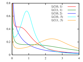
Probability density function
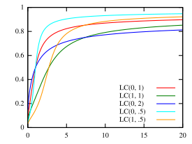
Cumulative distribution function
Parameters	$\mu$ (real) $\displaystyle \sigma >0\!$ (real)
Support	$\displaystyle x\in (0,+\infty )\!$
PDF	${1 \over x\pi }\left[{\sigma \over (\ln x-\mu )^{2}+\sigma ^{2}}\right],\ \ x>0$
CDF	${\frac {1}{\pi }}\arctan \left({\frac {\ln x-\mu }{\sigma }}\right)+{\frac {1}{2}},\ \ x>0$
Mean	infinite
Median	$e^{\mu }\,$
Variance	infinite
Skewness	does not exist
Excess kurtosis	does not exist
MGF	does not exist

In probability theory, a log-Cauchy distribution is a probability distribution of a random variable whose logarithm is distributed in accordance with a Cauchy distribution. If X is a random variable with a Cauchy distribution, then Y = exp(X) has a log-Cauchy distribution; likewise, if Y has a log-Cauchy distribution, then X = log(Y) has a Cauchy distribution.

Characterization

The log-Cauchy distribution is a special case of the log-t distribution where the degrees of freedom parameter is equal to 1.

Probability density function

The log-Cauchy distribution has the probability density function:

${\begin{aligned}f(x;\mu ,\sigma )&={\frac {1}{x\pi \sigma \left[1+\left({\frac {\ln x-\mu }{\sigma }}\right)^{2}\right]}},\ \ x>0\\&={1 \over x\pi }\left[{\sigma \over (\ln x-\mu )^{2}+\sigma ^{2}}\right],\ \ x>0\end{aligned}}$

where $\mu$ is a real number and $\sigma >0$. If $\sigma$ is known, the scale parameter is $e^{\mu }$. $\mu$ and $\sigma$ correspond to the location parameter and scale parameter of the associated Cauchy distribution. Some authors define $\mu$ and $\sigma$ as the location and scale parameters, respectively, of the log-Cauchy distribution.

For $\mu =0$ and $\sigma =1$, corresponding to a standard Cauchy distribution, the probability density function reduces to:

$f(x;0,1)={\frac {1}{x\pi (1+(\ln x)^{2})}},\ \ x>0$

Cumulative distribution function

The cumulative distribution function (cdf) when $\mu =0$ and $\sigma =1$ is:

$F(x;0,1)={\frac {1}{2}}+{\frac {1}{\pi }}\arctan(\ln x),\ \ x>0$

Survival function

The survival function when $\mu =0$ and $\sigma =1$ is:

$S(x;0,1)={\frac {1}{2}}-{\frac {1}{\pi }}\arctan(\ln x),\ \ x>0$

Hazard rate

The hazard rate when $\mu =0$ and $\sigma =1$ is:

$\lambda (x;0,1)=\left({\frac {1}{x\pi \left(1+\left(\ln x\right)^{2}\right)}}\left({\frac {1}{2}}-{\frac {1}{\pi }}\arctan(\ln x)\right)\right)^{-1},\ \ x>0$

The hazard rate decreases at the beginning and at the end of the distribution, but there may be an interval over which the hazard rate increases.

Properties

The log-Cauchy distribution is an example of a heavy-tailed distribution. Some authors regard it as a "super-heavy tailed" distribution, because it has a heavier tail than a Pareto distribution-type heavy tail, i.e., it has a logarithmically decaying tail. As with the Cauchy distribution, none of the non-trivial moments of the log-Cauchy distribution are finite. The mean is a moment so the log-Cauchy distribution does not have a defined mean or standard deviation.

The log-Cauchy distribution is infinitely divisible for some parameters but not for others. Like the lognormal distribution, log-t or log-Student distribution and Weibull distribution, the log-Cauchy distribution is a special case of the generalized beta distribution of the second kind. The log-Cauchy is actually a special case of the log-t distribution, similar to the Cauchy distribution being a special case of the Student's t distribution with 1 degree of freedom.

Since the Cauchy distribution is a stable distribution, the log-Cauchy distribution is a logstable distribution. Logstable distributions have poles at x=0.

Estimating parameters

The median of the natural logarithms of a sample is a robust estimator of $\mu$. The median absolute deviation of the natural logarithms of a sample is a robust estimator of $\sigma$.

Uses

In Bayesian statistics, the log-Cauchy distribution can be used to approximate the improper Jeffreys-Haldane density, 1/k, which is sometimes suggested as the prior distribution for k where k is a positive parameter being estimated. The log-Cauchy distribution can be used to model certain survival processes where significant outliers or extreme results may occur. An example of a process where a log-Cauchy distribution may be an appropriate model is the time between someone becoming infected with HIV and showing symptoms of the disease, which may be very long for some people. It has also been proposed as a model for species abundance patterns.

References

- ^ a b c d e f Olive, D.J. (June 23, 2008). "Applied Robust Statistics" (PDF). Southern Illinois University. p. 86. Archived from the original (PDF) on September 28, 2011. Retrieved 2011-10-18.
- ^ Olosunde, Akinlolu & Olofintuade, Sylvester (January 2022). "Some Inferential Problems from Log Student's T-distribution and its Multivariate Extension". Revista Colombiana de Estadística - Applied Statistics. 45 (1): 209–229. doi:10.15446/rce.v45n1.90672. Retrieved 2022-04-01.
{{cite journal}}: CS1 maint: multiple names: authors list (link) - ^ a b Lindsey, J.K. (2004). Statistical analysis of stochastic processes in time. Cambridge University Press. pp. 33, 50, 56, 62, 145. ISBN 978-0-521-83741-5.
- ^ a b c d Mode, C.J. & Sleeman, C.K. (2000). Stochastic processes in epidemiology: HIV/AIDS, other infectious diseases. World Scientific. pp. 29–37. ISBN 978-981-02-4097-4.
- ^ a b c d e f Marshall, A.W. & Olkin, I. (2007). Life distributions: structure of nonparametric, semiparametric, and parametric families. Springer. pp. 443–444. ISBN 978-0-387-20333-1.
- ^ a b Falk, M.; Hüsler, J. & Reiss, R. (2010). Laws of Small Numbers: Extremes and Rare Events. Springer. p. 80. ISBN 978-3-0348-0008-2.
- ^ Alves, M.I.F.; de Haan, L. & Neves, C. (March 10, 2006). "Statistical inference for heavy and super-heavy tailed distributions" (PDF). Archived from the original (PDF) on June 23, 2007.
- ^ "Moment". Mathworld. Retrieved 2011-10-19.
- ^ Wang, Y. "Trade, Human Capital and Technology Spillovers: An Industry Level Analysis". Carleton University: 14.
{{cite journal}}: Cite journal requires|journal=(help) - ^ Bondesson, L. (2003). "On the Lévy Measure of the Lognormal and LogCauchy Distributions". Methodology and Computing in Applied Probability: 243–256. Archived from the original on 2012-04-25. Retrieved 2011-10-18.
- ^ Knight, J. & Satchell, S. (2001). Return distributions in finance. Butterworth-Heinemann. p. 153. ISBN 978-0-7506-4751-9.
- ^ Kemp, M. (2009). Market consistency: model calibration in imperfect markets. Wiley. ISBN 978-0-470-77088-7.
- ^ MacDonald, J.B. (1981). "Measuring Income Inequality". In Taillie, C.; Patil, G.P.; Baldessari, B. (eds.). Statistical distributions in scientific work: proceedings of the NATO Advanced Study Institute. Springer. p. 169. ISBN 978-90-277-1334-6.
- ^ a b Kleiber, C. & Kotz, S. (2003). Statistical Size Distributions in Economics and Actuarial Science. Wiley. pp. 101–102, 110. ISBN 978-0-471-15064-0.
- ^ Panton, D.B. (May 1993). "Distribution function values for logstable distributions". Computers & Mathematics with Applications. 25 (9): 17–24. doi:10.1016/0898-1221(93)90128-I.
- ^ Good, I.J. (1983). Good thinking: the foundations of probability and its applications. University of Minnesota Press. p. 102. ISBN 978-0-8166-1142-3.
- ^ Chen, M. (2010). Frontiers of Statistical Decision Making and Bayesian Analysis. Springer. p. 12. ISBN 978-1-4419-6943-9.
- ^ Lindsey, J.K.; Jones, B. & Jarvis, P. (September 2001). "Some statistical issues in modelling pharmacokinetic data". Statistics in Medicine. 20 (17–18): 2775–278. doi:10.1002/sim.742. PMID 11523082. S2CID 41887351.
- ^ Zuo-Yun, Y.; et al. (June 2005). "LogCauchy, log-sech and lognormal distributions of species abundances in forest communities". Ecological Modelling. 184 (2–4): 329–340. doi:10.1016/j.ecolmodel.2004.10.011.
![{\displaystyle {1 \over x\pi }\left[{\sigma \over (\ln x-\mu )^{2}+\sigma ^{2}}\right],\ \ x>0}](https://wikimedia.org/enwiki/api/rest_v1/media/math/render/svg/8ac7d87d9737a9d396f445dfeb9b4cff6c3d0a12)
![{\displaystyle {\begin{aligned}f(x;\mu ,\sigma )&={\frac {1}{x\pi \sigma \left[1+\left({\frac {\ln x-\mu }{\sigma }}\right)^{2}\right]}},\ \ x>0\\&={1 \over x\pi }\left[{\sigma \over (\ln x-\mu )^{2}+\sigma ^{2}}\right],\ \ x>0\end{aligned}}}](https://wikimedia.org/enwiki/api/rest_v1/media/math/render/svg/a188fc444184e191f4e0325b64a2fb201546adfe)